
In broad terms, there are two types of momentum factors: mean reversion and auto-correlation.
Mean reversion momentum factors are generally calculated over short time-periods and their predictive power dissipates quickly. They exploit short-term liquidity distortions and are usually analysed within well-defined risk groups. This type of investing is typically referred to as statistical arbitrage. Given the relatively short holding period, transaction costs need to be closely monitored and constrained.
Auto-correlation momentum factors exploit the tendency of past winners to continue outperforming and past losers to continue underperforming. They are calculated over longer time periods, typically 3 to 18 months. Based on Narasimhan Jegadeesh and Sheridan Titman’s seminal 1993 research paper, the optimal holding period roughly corresponds with the time period over which the momentum factor is calculated (eg 6 month holding period for a 6 month momentum factor).
The focus of this research note is on autocorrelation momentum factors. We incorporate elements of statistical arbitrage into our rebalancing process, but the momentum factors included in our stock selection process are of the auto-correlation variety.
Why Do Momentum Factors Work?
This is an interesting question because it directly contradicts the weak from of the Efficient Market Hypothesis (EMH). Given we’re practitioners rather than academics, we’re not fans of the EMH but it does seem strange that a simple strategy of buying past winners and selling past losers has consistently generated alpha. The data required to calculate momentum factors is readily available and hence any alpha should be arbitraged away.
The original explanation put forward to explain the autocorrelation momentum anomaly is based on the “disposition effect”. This represents the tendency for investors to sell winners to lock in gains and hold on to losers in the hope of recouping losses. This is a common behavioural bias which most investors can relate to and was first documented in 1985 by Kahnerman and Tversky.
More recently, a research paper published by Da et al. in 2014 proposes that autocorrelation momentum factors work because investors underreact to information arriving in small pieces. The boiling frog syndrome is used to describe this behavioural bias with investors underreacting to information which is delivered gradually over time without the shock and awe associated with a major event that attracts a lot of attention and publicity.
“Clean” Momentum
The momentum anomaly rationale provided by Da et al. was the inspiration for developing more sophisticated momentum factors which remove the impact of outliers and capture the underlying trend driving share price returns.
These “clean” momentum factors are calculated over different time periods, ranging from 3 months to 2 years.
We calculate factor performance based on a range of metrics, including rank ICs, fractile returns, decay rates, and pure factor returns (after controlling for key risk factor exposures). In each market in the Fund’s stock universe, and over different backtest periods, the clean momentum factors exhibit superior predictive power relative to total return factors.
The chart below shows the one-month rank IC for our 12 month “clean” momentum factor versus a 12- month total return factor in Australia. We have selected Australia as it is a market where simple total return factors, such as the trailing 12-month total return, have performed strongly.
Chart 1: 12 Month Clean Momentum vs 12 Month Total Return (Australia, Rank IC)
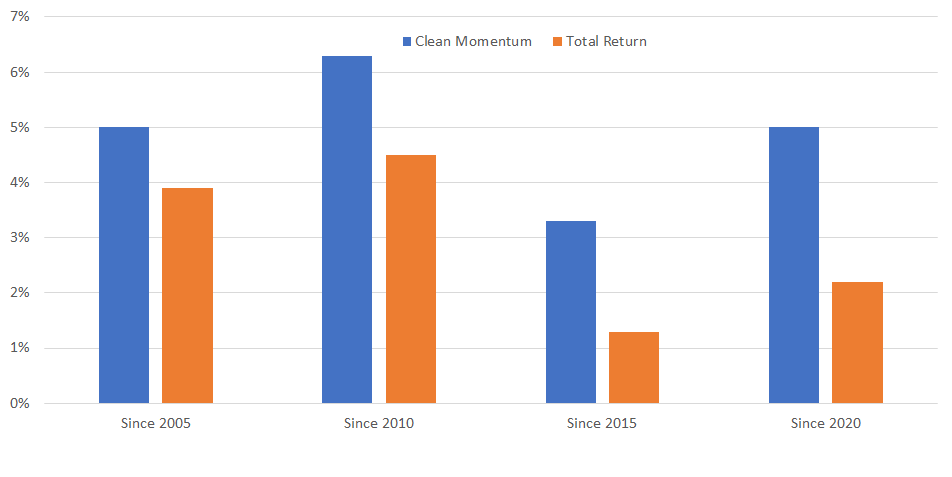
Source: FactSet, OQFM
To facilitate out-of-sample testing, we can also perform backtests across European equity markets and in the United States. Our backtests in these markets confirm the efficacy of the clean momentum factors.
Please contract us for more information on our backtest results, the methodology we use to calculate the clean momentum factors, and how we combine momentum factors over different time periods to calculate our composite momentum factor.
Comments